Introduction

Disparity Maps. A disparity map, often referred to as a depth map, is an image which contains depth information of every pixel stored in it. The term disparity in stereo vision refers to the apparent shift in pixel or motion in a pair of stereo images. Now a quick experiment to verify this would be to put an object (say a pencil) in front of your eyes. Observe the object with the right eye closed, and then at the same time quickly open your left eye and close your right eye. You would notice a shift in the object, this is what disparity basically means. Another thing you’ll notice is that objects far from your eyes shift less, and objects nearer shift more! This proves that disparity and depth have an inverse relationship. In this small experiment your eyes act as stereo camera system. In fact depth and disparity are related by the following equation

where $x$ and $x’$ are the x-coordinate of a point in the left image and right image respectively of a rectified stereo image pair. $f$ is the focal length of the camera, $B$ is the baseline, and $Z$ is the depth of that point in 3D space.

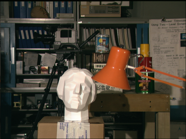
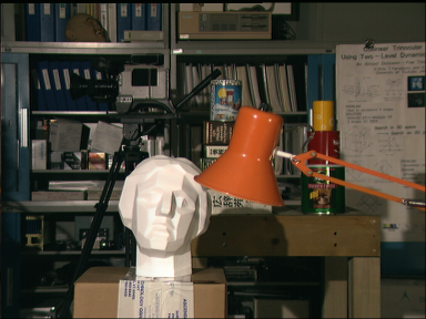
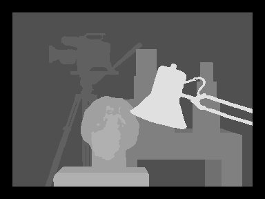
The disparity map shown in the above example is a grayscale image. Pixels which are colored white depict high disparity (low depth) and pixels which are coloured dark indicate low disparity (more depth). Generating accurate dense disparity maps is an active research area in computer vision. The Middlebury stereo evaluation dataset shows the current best methods for computing dense disparity maps. It is to be noted that most of the methods from that list are global methods which formulate a global optimization problem and tries to minimize a cost or energy. These methods take significant amount of computation time and power and may not be useful for real time systems, although they tend to be really accurate. In this article a local method for computing disparity maps is presented.

ORB Descriptors. ORB which stands for Oriented FAST and Rotated BRIEF is an efficient feature detection algorithm designed by Rublee et al. Their paper, ORB: an efficient alternative to SIFT or SURF, is widely used by the computer vision community for various tasks. ORB basically finds a number of key points in an image and computes their descriptors to be matched in another image which may be rotated or scaled. In our case all the pixels in our image would be key points i.e. we will manually set all pixels (x, y) as key points by calling the OpenCV key point constructor as KeyPoint(x, y, 1) where 1 is the diameter of the key point. Once all the key points are set, a descriptor for each key point is computed. These descriptors are a 32x1 integer vector representing each pixel. To find the point correspondences, a window based descriptor matching method is implemented.

Stereo Calibration and Rectification

Before proceeding to generate a dense disparity map, it is required to calibrate a pair of stereo cameras and rectify the stereo images so that the epipolar lines become horizontal scan lines.

Epipolar Matching

The epipolar constraint states that the correspondence of any point in one image is bound to lie on a particular line, called the epipolar line, in the other image. For rectified images these lines become horizontal and are called scan lines. A square window (target window) is slid over the epipolar line and the sum of the absolute differences (SAD) of each descriptor between the target window and the current window is computed. Among all such target windows the one with the minimum cost is chosen and the center of that window is the corresponding pixel. Note that, intensity differences are not being calculated for each pixel, instead the L1 norm of the difference vector of orb descriptors will be computed.

Cost Function. Since the epipolar are horizontal scan lines, we don’t have to worry about the y-coordinate. Let $C(x,d)$ be the cost of a pixel in the left image having disparity $d$. A pixel having disparity $d$ means the corresponding pixel in the right image has its x-coordinate as $x-d$. Then the best disparity $d_x$ is selected using a winner-take-all (WTA) scheme.

where $D_x = [0,d_{\max}-1]$ is the set of possible disparity values. The cost function $C(x,d)$ is defined as follows

where $W(x)$ is the window around the pixel $x$, $D_1(i,j)$ is the descriptor for the pixel $(i,j)$ in the left image and similarly $D_2$ is the descriptor for the corresponding pixel in the right image.

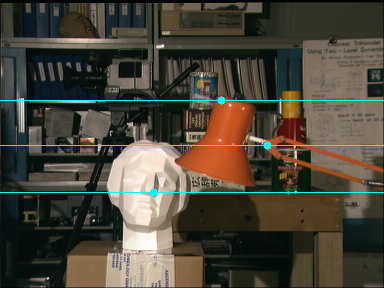
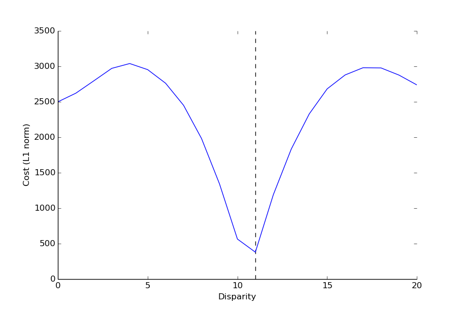
The cost graph shown above depicts a single minimum. This indicates a high confidence match. In some cases there might be multiple minima, which usually results in low confidence incorrect matches. This usually occurs in textureless regions. Why? Think about it!

Left-Right Correspondence Check. This technique is used to do away with matching errors, especially in occluded regions. The disparity for pixel $(x,y)$ in the left image is first determined, say it is $d_1$. Then the disparity $d_2$ for pixel $(x-d_1,y)$ in the right image is calculated by drawing its epipolar line in the left image. The match is determined as valid/confident if $d_1$ and $d_2$ are almost equal i.e. if

where $\delta$ is some threshold. Usually $\delta < 5$. The left-right correspondence check is implemented while generating the dense disparity map.

Epipolar matching: C++/OpenCV implementation

#include <iostream>
#include <opencv2/opencv.hpp>
#include <opencv2/features2d/features2d.hpp>
#include <fstream>

using namespace cv;
using namespace std;

Mat img_left, img_right, img_left_disp, img_right_disp;
Mat img_left_desc, img_right_desc;
vector< KeyPoint > kpl, kpr;

Declare all necessary variables. img_left and img_right stores the rectified stereo images. img_left_desc and img_right_desc stores the descriptor values of all the key points. kpl and kpr stores the left and right image key points respectively.

bool isLeftKeyPoint(int i, int j) {
  int n = kpl.size();
  return (i >= kpl[0].pt.x && i <= kpl[n-1].pt.x
          && j >= kpl[0].pt.y && j <= kpl[n-1].pt.y);
}

bool isRightKeyPoint(int i, int j) {
  int n = kpr.size();
  return (i >= kpr[0].pt.x && i <= kpr[n-1].pt.x
          && j >= kpr[0].pt.y && j <= kpr[n-1].pt.y);
}

Create two helper functions isLeftKeyPoint and isRightKeyPoint to check if pixel $(i,j)$ is a valid key point.

Note: Not all pixels are valid key points i.e. descriptor values do not exist for them. These are pixels which are close to the edge of the image.

void cacheDescriptorVals() {
  OrbDescriptorExtractor extractor;
  for (int i = 0; i < img_left.cols; i++) {
    for (int j = 0; j < img_left.rows; j++) {
      kpl.push_back(KeyPoint(i,j,1));
      kpr.push_back(KeyPoint(i,j,1));
    }
  }
  extractor.compute(img_left, kpl, img_left_desc);
  extractor.compute(img_right, kpr, img_right_desc);
}

Precompute descriptor values for all valid key points (both left and right) using OrbDescriptorExtractor. We manually set key points as KeyPoint(i, j, 1) because we require descriptors for all pixels. If we let ORB compute key points, only a sparse set of key points will be returned.

long costF(const Mat& left, const Mat& right) {
  long cost = 0;
  for (int i = 0; i < 32; i++) {
    cost += abs(left.at<uchar>(0,i)-right.at<uchar>(0,i));
  }
  return cost;
}

Define a cost function costF to compute the L1 norm of two descriptors. Here left and right are two descriptors of a left and right image pixel respectively. Since descriptors are 32x1 vectors we sum the absolute value of their term by term difference to find the cost.

int getCorresPoint(Point p, Mat& img, int ndisp) {
  ofstream mfile;
  mfile.open("cost.txt");
  int w = 5;
  long minCost = 1e9;
  int chosen_i = 0;
  int x0r = kpr[0].pt.x;
  int y0r = kpr[0].pt.y;
  int ynr = kpr[kpr.size()-1].pt.y;
  int x0l = kpl[0].pt.x;
  int y0l = kpl[0].pt.y;
  int ynl = kpl[kpl.size()-1].pt.y;
  for (int i = p.x-ndisp; i <= p.x; i++) {
    long cost = -1;
    for (int j = -w; j <= w; j++) {
      for (int k = -w; k <= w; k++) {
        if (!isLeftKeyPoint(p.x+j, p.y+k) || !isRightKeyPoint(i+j, p.y+k))
          continue;
        int idxl = (p.x+j-x0l)*(ynl-y0l+1)+(p.y+k-y0l);
        int idxr = (i+j-x0r)*(ynr-y0r+1)+(p.y+k-y0r);
        cost += costF(img_left_desc.row(idxl), img_right_desc.row(idxr));
      }
    }
    cost = cost / ((2*w+1)*(2*w+1));
    mfile << (p.x-i) << " " << cost << endl;
    if (cost < minCost) {
      minCost = cost;
      chosen_i = i;
    }
  }
  cout << "minCost: " << minCost << endl;
  return chosen_i;
}

getCorresPoint returns the corresponding matched x-coordinate in the right image, given a point p in the left image. w is the size of the window to be slid across the epipolar line. ndisp is the maximum disparity / number of disparities for the stereo image pair. chosen_i is the current best pixel in the right image. idxl is the index of the descriptor of pixel $(x,y)$ in img_left_desc. It’s the same for idxr.

$x_{0l}$ and $y_{0l}$ are the x and y coordinates of the first key point in kpl respectively. $y_{nl}$ is the y-coordinate of the last key point in kpl. The key point descriptors are stored in column major format, hence the formula above is used to access them.

void mouseClickLeft(int event, int x, int y, int flags, void* userdata) {
  if (event == EVENT_LBUTTONDOWN) {
    if (!isLeftKeyPoint(x,y))
      return;
    int right_i = getCorresPoint(Point(x,y), img_right, 20);
    Scalar color = Scalar(255,255,0);
    circle(img_left_disp, Point(x,y), 4, color, -1, 8, 0);
    circle(img_right_disp, Point(right_i,y), 4, color, -1, 8, 0);
    line(img_right_disp, Point(0,y), Point(img_right.cols,y), 
         color, 1, 8, 0);
    cout << "Left: " << x << " Right: " << right_i << endl;
  }
}

Create a callback function for a left click on the left image. This will trigger the getCorresPoint function for the clicked pixel $(x,y)$. Circles are drawn on both images to visually show the correspondences, the epipolar line is drawn too. Note that all the visualizations are done on img_left_disp and img_right_disp.

int main(int argc, char const *argv[])
{
  img_left = imread(argv[1]);
  img_right = imread(argv[2]);
  img_left_disp = imread(argv[1]);
  img_right_disp = imread(argv[2]);
  cacheDescriptorVals();
  namedWindow("IMG-LEFT", 1);
  namedWindow("IMG-RIGHT", 1);
  setMouseCallback("IMG-LEFT", mouseClickLeft, NULL);
  while (1) {
    imshow("IMG-LEFT", img_left_disp);
    imshow("IMG-RIGHT", img_right_disp);
    if (waitKey(30) > 0) {
      break;
    }
  }
  return 0;
}

Finally the main function takes two rectified images as input and calls all the necessary functions to implement the epipolar matching.

Find the full code here: https://github.com/sourishg/disparity-map/blob/master/epipolar.cpp

Generating dense disparity maps: C++/OpenCV implementation

The idea is to extend the epipolar matching for all pixels in the left image. Hence much of the previous code is reused. The final output is a grayscale showing the various disparity levels of each pixel. If a pixel $(x,y)$ has disparity $d$, then the grayscale intensity of the corresponding pixel is $\frac{255 \times d}{d_{\max}}$.

void computeDisparityMapORB(int ndisp) {
  img_disp = Mat(img_left.rows, img_left.cols, CV_8UC1, Scalar(0));
  int x0 = kpl[0].pt.x;
  int y0 = kpl[0].pt.y;
  int yn = kpl[kpl.size()-1].pt.y;
  for (int i = 0; i < img_left.cols; i++) {
    for (int j = 0; j < img_left.rows; j++) {
      cout << i << ", " << j << endl;
      if (!isLeftKeyPoint(i,j))
        continue;
      int right_i = getCorresPointRight(Point(i,j), ndisp);
      // left-right check
      int left_i = getCorresPointLeft(Point(right_i,j), ndisp);
      if (abs(left_i-i) > 5)
        continue;
      int disparity = abs(i - right_i);
      img_disp.at<uchar>(j,i) = disparity * (255. / ndisp);
    }
  }
}

This is a very simple function which makes use of getCorresPointRight and getCorresPointLeft to find the left and right disparity respectively. If the left-right correspondence check is passed for pixel $(i,j)$ then the corresponding grayscale intensity is set in the disparity image, otherwise it is coloured black.

int main(int argc, char const *argv[])
{
  img_left = imread(argv[1], 1);
  img_right = imread(argv[2], 1);
  cacheDescriptorVals();
  computeDisparityMapORB(20);
  //namedWindow("IMG-LEFT", 1);
  //namedWindow("IMG-RIGHT", 1);
  while (1) {
    imshow("IMG-LEFT", img_left);
    imshow("IMG-RIGHT", img_right);
    imshow("IMG-DISP", img_disp);
    if (waitKey(30) > 0) {
      imwrite(argv[3], img_disp);
      break;
    }
  }
  return 0;
}

The main function caches the descriptor values and then calls the computeDisparityMapORB function to generate the dense disparity map.

Find the full code here: https://github.com/sourishg/disparity-map/blob/master/disparity-orb.cpp

Results

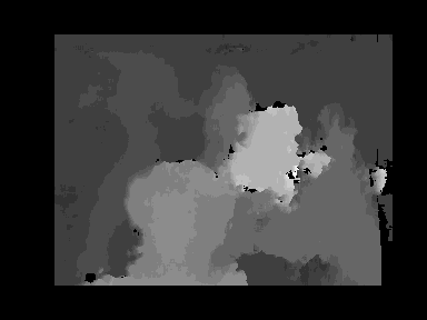
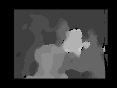
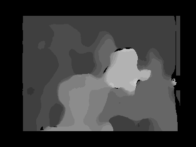
Tsukuba Stereo Pair. The images shown above are the results of ORB-based disparity matching. As it is clearly seen the results are not as good as the ground truth but it is good enough for local window-based matcher. It can be clearly seen that the rods/support of the lamp is not correctly matched and the tripod stand behind is also not properly depicted. But the overall structure/shape of the scene is retained to a fair extent. Also the effect of window-size can be seen. The first image is a bit noisy due to a lesser window-size whereas the the other two are a bit smoother and patchy because of a greater window-size.

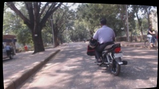
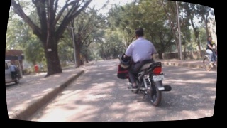
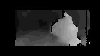
IIT KGP Dataset. This is an outdoor data set. The above stereo pair was collected using two Logitech C920s. Although the disparity map looks fair but there are issues – disparities for the ground plane is not smooth enough. The 3D reconstruction would yield a rough ground plane which is not good if someone is using stereo for obstacle avoidance. This is one of the drawbacks of local methods for generating dense disparity maps.

More tools here: https://github.com/sourishg/disparity-map