Introduction

This article is a tutorial of the code implemented in the repository stereo-dense-reconstruction. The theory is not covered in detail, so some basic reading on the topic is suggested before one delves into the code. This ROS package computes dense disparity maps using LIBELAS and converts them into 3D point clouds. The method for generation of disparity maps can be changed based on user preferences. I had written an article on generating dense disparity maps using ORB descriptors earlier. That method can be implemented real time by using optimized code and parallelization.

An overview of the working code can be seen in the above video. Generation of dense disparity maps and the resulting point clouds is shown. The visualizations are shown in rviz. Towards the end of the video, point cloud transformation is demonstrated using rqt_reconfigure.

Stereo Calibration

A calibrated pair of stereo cameras is required for dense reconstruction. The calibration file is stored as a YAML file containing the following information about the stereo cameras:

See a sample calibration file. A YAML calibration file can be generated by using this stereo camera calibration tool. For more information see this detailed tutorial on stereo camera calibration.

Although we require only the matrices mentioned in the above table, the sample calibration file contains other matrices found after rectification (e.g., P1, P2, Q etc.). These matrices are found by OpenCV’s stereoRectify function and they depend on the output image resolution of the rectified stereo images. Hence it is better to run stereoRectify online than storing those matrices in a calibration file. This gives us the flexibility to work at different image resolutions.

The use of XR and XT matrices is explained later. For initial values XR can be set as the $3 \times 3$ identity matrix while XT can be set as the $3 \times 1$ zero vector.

Stereo Rectification

Disparity maps are generated from rectified stereo images. The raw stereo images should be published by a topic which publishes messages of the type sensor_msgs/Image. The code for rectification of stereo images is implemented in src/stereo_rectify.cpp.

Mat XR, XT, Q, P1, P2;
Mat R1, R2, K1, K2, D1, D2, R;
Vec3d T;
Mat lmapx, lmapy, rmapx, rmapy;
FileStorage calib_file;
Size out_img_size(320, 240);
Size calib_img_size(640, 480);

image_transport::Publisher pub_img_left;
image_transport::Publisher pub_img_right;

Declare all the calibration matrices as Mat variables. calib_img_size is the resolution of the images used for stereo calibration. out_img_size is the output resolution of the rectified images. This can be set at our own will. Lower resolution images require less computation time for dense reconstruction. pub_img_left and pub_img_right are the publishers for the rectified images. The output images are published as a sensor_msgs/CompressedImage message. This is helpful while collecting large datasets, so that file size is reduced.

void undistortRectifyImage(Mat& src, Mat& dst, FileStorage& calib_file, int
left = 1) {
  if (left == 1) {
    remap(src, dst, lmapx, lmapy, cv::INTER_LINEAR);
  } else {
    remap(src, dst, rmapx, rmapy, cv::INTER_LINEAR);
  }
}

This function undistorts and rectifies the src image into dst. The homographic mappings lmapx, lmapy, rmapx, and rmapy are found from OpenCV’s initUndistortRectifyMap function.

void findRectificationMap(FileStorage& calib_file, Size finalSize) {
  Rect validRoi[2];
  cout << "starting rectification" << endl;
  stereoRectify(K1, D1, K2, D2, calib_img_size, R, Mat(T), R1, R2, P1, P2, Q,
                CV_CALIB_ZERO_DISPARITY, 0, finalSize, &validRoi[0],
&validRoi[1]);
  cout << "done rectification" << endl;
  cv::initUndistortRectifyMap(K1, D1, R1, P1, finalSize, CV_32F, lmapx,
lmapy);
  cv::initUndistortRectifyMap(K2, D2, R2, P2, finalSize, CV_32F, rmapx,
rmapy);
}

This function computes all the projection matrices and the rectification transformations using the stereoRectify and initUndistortRectifyMap functions respectively.

void imgLeftCallback(const sensor_msgs::ImageConstPtr& msg) {
  try
  {
    Mat tmp = cv_bridge::toCvShare(msg, "bgr8")->image;
    if (tmp.empty()) return;
    Mat dst;
    undistortRectifyImage(tmp, dst, calib_file, 1);
    sensor_msgs::ImagePtr img_left;
    img_left = cv_bridge::CvImage(msg->header, "bgr8",
dst).toImageMsg();
    pub_img_left.publish(img_left);
  }
  catch (cv_bridge::Exception& e)
  {
  }
}

This callback function takes a raw stereo (left) image as input. Then it undistorts and rectifies the image using the functions defined above and publishes on the rectified image topic using pub_img_left. Similarly imgRightCallback is defined for the right stereo image.

int main(int argc, char** argv) {
  ros::init(argc, argv, "stereo_rectify");
  ros::NodeHandle nh;
  image_transport::ImageTransport it(nh);

  calib_file = FileStorage(argv[3], FileStorage::READ);
  calib_file["K1"] >> K1;
  calib_file["K2"] >> K2;
  calib_file["D1"] >> D1;
  calib_file["D2"] >> D2;
  calib_file["R"] >> R;
  calib_file["T"] >> T;
  findRectificationMap(calib_file, out_img_size);

  ros::Subscriber sub_img_left = nh.subscribe(argv[1], 1, imgLeftCallback);
  ros::Subscriber sub_img_right = nh.subscribe(argv[2], 1, imgRightCallback);

  pub_img_left = it.advertise("/camera_left_rect/image_color", 1);
  pub_img_right = it.advertise("/camera_right_rect/image_color", 1);

  ros::spin();
  return 0;
}

In the main function, the stereo calibration information is read into calib_file. sub_img_left and sub_img_right subscribes to the topics publishing the raw stereo image data. The rectified output images are published to the following topics:

• /camera_left_rect/image_color
• /camera_right_rect/image_color

The ros node can be run as

$ rosrun stereo_dense_reconstruction stereo_rectify [/camera/left/topic] [/camera/right/topic] [path/to/calib/file.yml]

Dense 3D Reconstruction

Generating dense 3D reconstructions involve two major steps: (1) computing a disparity map (2) converting the disparity map into a 3D point cloud. The code for dense reconstruction is implemented in src/dense_reconstruction.cpp.

Having time synced stereo images is important for generating accurate disparity maps. To sync the left and right image messages by their header time stamps, ApproximateTime is used. The procedure is implemented in the main function of src/dense_reconstruction.cpp.

message_filters::Subscriber<sensor_msgs::CompressedImage> sub_img_left(nh, "/camera_left_rect/image_color/compressed", 1);
message_filters::Subscriber<sensor_msgs::CompressedImage> sub_img_right(nh, "/camera_right_rect/image_color/compressed", 1);

typedef message_filters::sync_policies::ApproximateTime<sensor_msgs::CompressedImage, sensor_msgs::CompressedImage> SyncPolicy;
message_filters::Synchronizer<SyncPolicy> sync(SyncPolicy(10), sub_img_left, sub_img_right);
sync.registerCallback(boost::bind(&imgCallback, _1, _2));

This syncs the two rectified image topics, and the callback function imgCallback receives the time synced messages.

Disparity Maps using LIBELAS

LIBELAS (Efficient Large-Scale Stereo Matching) is a great open source software for generating dense disparity maps. It does not use global optimization techniques and yet produces great results at almost real time. More information about ELAS can be found here.

Mat generateDisparityMap(Mat& left, Mat& right) {
  if (left.empty() || right.empty())
    return left;
  const Size imsize = left.size();
  const int32_t dims[3] = {imsize.width,imsize.height,imsize.width};
  Mat leftdpf = Mat::zeros(imsize, CV_32F);
  Mat rightdpf = Mat::zeros(imsize, CV_32F);

  Elas::parameters param;
  param.postprocess_only_left = true;
  Elas elas(param);
  elas.process(left.data,right.data,leftdpf.ptr<float>(0),
               rightdpf.ptr<float>(0),dims);

  Mat show = Mat(out_img_size, CV_8UC1, Scalar(0));
  leftdpf.convertTo(show, CV_8U, 1.);
  if (!show.empty()) {
    sensor_msgs::ImagePtr disp_msg;
    disp_msg = cv_bridge::CvImage(std_msgs::Header(), "mono8",
show).toImageMsg();
    dmap_pub.publish(disp_msg);
  }
  return show;
}

This function computes the dense disparity map using LIBELAS, and publishes it as a 8-bit grayscale image to the topic /camera_left_rect/disparity_map. The disparity map is constructed with the left image as reference. The parameters for LIBELAS can be changed in the file src/elas/elas.h.

Any method other than LIBELAS can be implemented inside the generateDisparityMap function to generate disparity maps. One can use OpenCV’s StereoBM class as well. The output should be a 8-bit grayscale image.

3D Reconstruction

Given a disparity map, a corresponding 3D point cloud can be easily constructed. The Q matrix stored in the calibration file is used for this conversion. The reconstruction is mathematically expressed by the following matrix equation.

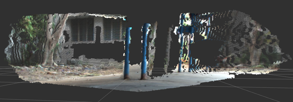
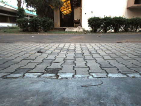
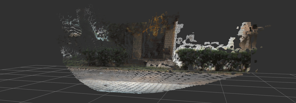
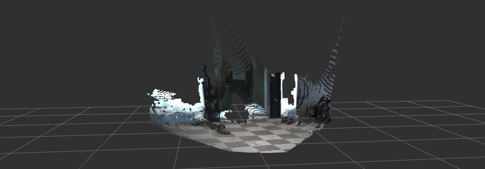
where $(X,Y,Z,W)^\top$ denotes the 3D point in homogeneous coordinates. $d(x,y)$ is the disparity of a point $(x,y)$ in the left image. The $4 \times 4$ matrix denotes the Q matrix. This matrix multiplication in homogeneous coordinates is implemented in the publishPointCloud function. It publishes a sensor_msgs/PointCloud message to the topic camera_left_rect/point_cloud. The point cloud generated is in the reference frame of the left camera. Hence a transformation (XR, XT) is applied to transform the point cloud into a different reference frame (as required by the user). The transformation equation is as follows

where $P_A$ is a point in reference frame $A$, $P_B$ is a point in the reference frame $B$. $R$ and $T$ denote the rotation and translation matrices respectively. In this case $R$ = XR and $T$ = XT. Figure 1 shows some visualizations of the resulting point clouds from dense disparity maps.

Run the dense reconstruction node as

$ rosrun stereo_dense_reconstruction dense_reconstruction [path/to/calib/file.yml]

Visualize the point cloud in rviz

$ rosrun rviz rviz

Point Cloud Transformation

For ground robots with mounted stereo cameras, usually the point clouds are formed in the reference frame of the left camera. Often the point clouds need to be transformed to a different frame e.g., a reference frame with the origin at the centre of rotation of the robot projected on to the ground plane. These transformations are hard to calculate mathematically. Hence it is easier to find these transformations visually, if the geometry of the scene is known.

The transformation from one reference frame to another is represented by the rotation matrix XR and the translation vector XT. XR can be decomposed into Euler angles ($\phi_x, \phi_y, \phi_z$) while XT contains the translation values in the $X,Y,$ and $Z$ direction. A config file cfg/CamToRobotCalibParams.cfg stores these six values. The config file is bound with the dense_reconstruction node using dynamic_reconfigure.

dynamic_reconfigure::Server<stereo_dense_reconstruction::
CamToRobotCalibParamsConfig> server;
dynamic_reconfigure::Server<stereo_dense_reconstruction::
CamToRobotCalibParamsConfig>::CallbackType f;

f = boost::bind(&paramsCallback, _1, _2);
server.setCallback(f);

The above piece of code implements dynamic_reconfigure to configure the transformation parameters.

Mat composeRotationCamToRobot(float x, float y, float z) {
  Mat X = Mat::eye(3, 3, CV_64FC1);
  Mat Y = Mat::eye(3, 3, CV_64FC1);
  Mat Z = Mat::eye(3, 3, CV_64FC1);

  X.at<double>(1,1) = cos(x);
  X.at<double>(1,2) = -sin(x);
  X.at<double>(2,1) = sin(x);
  X.at<double>(2,2) = cos(x);

  Y.at<double>(0,0) = cos(y);
  Y.at<double>(0,2) = sin(y);
  Y.at<double>(2,0) = -sin(y);
  Y.at<double>(2,2) = cos(y);

  Z.at<double>(0,0) = cos(z);
  Z.at<double>(0,1) = -sin(z);
  Z.at<double>(1,0) = sin(z);
  Z.at<double>(1,1) = cos(z);

  return Z*Y*X;
}

Mat composeTranslationCamToRobot(float x, float y, float z) {
  return (Mat_<double>(3,1) << x, y, z);
}

The above two functions are used to compose the matrices XR and XT. composeRotationCamToRobot finds a rotation matrix from three Euler angles by the $ZYX$ convention. composeTranslationCamToRobot returns a $3\times 1$ translation matrix.

Initially, the values of XR and XT in the calibration file were the $3\times 3$ identity matrix and the $3\times 1$ zero matrix. The function debugCamToRobotTransformation(XR, XT) can be used to dynamically change the values of XR and XT with the help of dynamic_reconfigure. If the desired transformation is found, the resulting values of XR and XT can be updated in the calibration file. To modify the transformation values start dynamic_reconfigure by

$ rosrun rqt_reconfigure rqt_reconfigure

Refer to the video in the Introduction section to have a better understanding of how the point cloud transformation works. It is shown towards the end of the video.

Build and Run

Clone the repository stereo-dense-reconstruction in your ros catkin workspace. Build using catkin_make. Further instructions on running each node is given in the README of the repository.

References and Related Stuff

• Stereo Camera Calibration
• LIBELAS webpage
• Efficient Large-Scale Stereo Matching (paper)
• elas_ros (another implementation of ELAS on ROS)
• Finding 3D transformations